Week 7: Fingerprint Recognition

This is a belated post. The group was occupied with the work associated with the arrival of the fingerprint scanner, as well as working out the kinks of the existing code, that it forgot to publish a status update on the blog. However, the following is a documentation of the work during Week 7.

 

The fingerprint scanner arrived and we have been able to use it to take pictures of our fingerprints. Up to this point, the code for fingerprint analysis had been written using sample fingerprints. Now, the group is able to take its own fingerprints, and will intergrate these pictures into the existing code.

 

Additionally, the group had identified a new problem; it needs to integrate the software that came with the fingerprint scanner, which tells the scanner to take and save a picture, into the user log on screen. This is necessary so the user can take a picture of his/her thumb, so that it can be analyzed and compared with the test data base. This problem will need to be worked on in the future weeks.

Figure 1: Picture of FS80 USB 2.0 finerprint scanner.  

 

 

Figure 2: Fingerprint taken by fingerprint scanner mentioned above.

 

The code written that is intended to extract and isolate the minutiae of the swirls intrinsic to fingerprints needs some work to successfully match one fingerprint to its corresponding match in the test data base.

 

Figure 3:

Minutiae Extraction of Fingerprint Images Using Thinning Algorithm





Week 9 - Facial Recognition Updates

This belated post details progress made in the facial recognition component of the project. The facial recognition algorithm has been incorporated into the GUI and a timer has been implemented to cross-reference the video feed from the webcam to the training database every 0.1 seconds. This way, the user does not have to wait for the camera to take his/her photo. Instead, all of the processing is done automatically. A similar approach will be implemented for the fingerprint algorithm as shall be discussed in future blog posts.

The GUI has also been expanded to full-screen using the undocumented features of Java in MATLAB. The ancestor to the MATLAB frame is called and the JavaFrame is diposed; thereafter, the setUndecorated property is modified and the components are repacked and displayed. Other minor GUI changes and fixes have been made to improve the look-and-feel of the application.

Week 8 Voice Recognition

This week, the voice recognition portion of the project was completed and is being tested.  As touched upon earlier, the code consists of two files.  One- voicerecord.m and the other voicetest.m.  

1. The first file asks the user to record their name ten times giving them 2 seconds each time in succession.  After this, the database is setup and these 10 files are saved and archived in the Matlab director as .wav files.  Processing of these files is done in the next file.
2. Voicetest.m is the file where the majority of the project's processing takes place.  First, the ten files recorded earlier are prepared and formed into a matrix and transformed using the FFT.  A series of commands primes this matrix for comparison to the test recording.  Eventually, the person trying to gain access is asked to record their name this is immediately transformed (FFT).  Once the sample, and the saved recordings are in the frequency domain, they are compared using Chebyshev's Rule.  Simply, the rule states that at least 89% of the data values belonging to the identical set must be within 3 standard deviations of the mean.  Therefore, if the sample is so far off from the the saved set, it can be assumed that it is not part of the set, i.e. it is a different person.  If, however, it does fall in 3 standard deviations then it must be the same individual. 

Week 6 Voice Recognition Update

Development

Development of the Voice Recognition module is nearly halfway complete.  Initially, an overview of the process for the final algorithm was planned and is as follows:

1. The user creates the training database by recording 10 samples of he/she saying an arbirtray string sequence. 
2. Matlab converts, analyzes (converts from time to frequencey domain via Fast Fourier Transform (FFT)), and saves these as .wav files.
3. When the user tries to login he is prompted to repeat the certain sequence.
4. Matlab conducts FFT on the sample and then compares it to saved file top determine users identity.

http://www.osu-tulsa.okstate.edu/istr/blockdiagramsgrad.jpg

At this point, progress is on fine tuning step 3 and 1 and 2 have been completed. So far, the project consists of two Matlab (.m) files that have to be executed separately.   One for establishing identity and the other for testing it. 

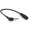
To test and verify outcome, a standard PC microphone manufactured by General Electric is being used.



http://ecx.images-amazon.com/images/I/21H7wzsa2eL._SL500_SS100_.jpg

A Look at Fourier Analysis

At the core of the algorithm is the Fourier Analysis.   A common tool used today, it was developed by the mathematician Joseph Fourier.  Fourier proved that any continuous function could be produced as an infinite sum of sine and cosine waves.  Using this information we can breakdown sound into its components and systematically analyze it. 

To accomplish this Matlab will be programmed to convert the sound wave from the time domain to the frequency domain as shown below:


http://hyperphysics.phy-astr.gsu.edu/hbase/audio/Fourier.html#c1

This picture shows the amplitudes of the individual components of the sound file displayed against their frequency.  It illustrates the power of a Fourier Transform in dealing with sound waves.

In summary, progress of the voice recognition module is proceeding as planned in the proposal.

Week 6 Updates - Face Recognition, Fingerprint, and Voice

The GUI was successfully developed using the MATLAB GUIDE template. The design was made to model a Windows 7 Login Screen and will appear before a user is able to log into the computer. A snapshot of the GUI in development can be seen below in Figure 1:

Figure 1. Windows 7 Login Screen Developed in MATLAB

The GUI was developed using the MATLAB environment and can be seen clearly in Figure 2.

Figure 2. MATLAB GUIDE Figure for Developing Windows 7 GUI

In place of the user image icon, a live video feed will be implemented so that the user can take a photo and access the account using biometric features.

Fingerprint Recognition
Minutiae extraction is complete and analysis techniques are being pursued and researched immediately.

Fingerprint Scanner
The fingerprint scanner has been ordered and will arrive within 2-5 business days. Testing will commence once the scanner has arrived and been integrated with MATLAB.

Week 5 Fingerprint Recognition Progress

Sources were used to find working algorithms to detect minutiae, patterns on fingerprints that are present in all fingerprints, differing in location on the print. Minutiae were extracted through a built in MATLAB algorithm that searches for designated patterns. Using thinned binary images of fingerprints, creating the patterns to look for was simple. 3x3 matrices including the search patterns were created and utilized in the search process. Once found, the minutiae were displayed on a figure, showing their relative locations.

Week 4 - Face Recognition Walkthrough

This week, we were able to advance on the face recognition component of the biometric recognition project. The steps for the MATLAB algorithm (pseudocode) are given below. In addition, we have decided on a fingerprint scanner and advanced with minutiae analysis of fingerprinting and Fourier analysis of voice.

1. Create a test database. Take a picture and convert it into grayscale to reduce the number of channels (R, G, B).

2. Then, reduce into a 1-D vector because all images share this property (R^m).

3. Add every "reshaped" vector to a matrix known as the "test" matrix of dimensions mxn concatenating vertically.

4. Taking this mxn matrix, take the mean along every row and output a column vector averaging every pixel in all 20 images.

5. Creating a new matrix, known as the SCATTER MATRIX, every individual column is subtracted by the mean vector (R^m) evaluated before.

6. The SCATTER MATRIX has dimensions mxn.

7. Because the SCATTER MATRIX is not necessarily square, it can be multiplied by its transpose to create a square matrix. It is known that the maximum number of eigenvalues for a mxn matrix (non-square) is min(m-1, n-1). Therefore, new eigenvalues will not be generated just because the square matrix with larger dimensions is chosen.

8. The objective is to make the process minimally computationally expensive. Because m is the number of pixels and n is the number of images, left-transposition yields nxm x mxn = nxn matrix. Right-transposition yields mxn x nxm = mxm, which is considerably larger than nxn. Therefore, nxn is the best choice.

9. After finding the eigenvalues and eigenvectors of nxn, the eigenfaces is a measure of how much faces differ from the mean face based on the data set. These eigenfaces are not unique to the faces used to compile them, but will be projected onto the original images themselves to determine how “different” an image is from others.

10. Once the eigenfaces have been computed, this matrix has at most nx(n-1) dimensions.

11. Once the eigenface matrix has been obtained (it has only numerical value and is in the eigenspace), it can be projected into imagespace by multiplying into the original grayscale matrix of pixels. This process has essentially extracted the principal components, hence the name PCA, that are unique to individuals such as the hairline, where the nose is, where the mouth is, etc. The background details become trivial because they are averaged with the mean face (a green-screen would be ideal and will be implemented in the final design).

12. The scatter of the test image will be obtained by subtracting from the mean of all images in the database. Multiplying by the eigenface matrix yields a “feature vector” that contains the principal component details.

13. The total Euclidean distance in imagespace between the projected test image and the training images is computed for every image. The image with smallest scatter when compared to the appropriate image is the best match!